This is the #2 post in my series of posts about approximate Bayesian Inference (BI) where I will be talking about Variational Inference. If you do not understand most of the things here, I would recommend reading my previous post and/or the references.
Here is the outline of the blog posts of this series on BI:
- Introduction.
- Variational Inference (1) - Intro & Mean-Field Approximation (you are here).
The outline will be updated in time as I post my drafts.
The content in this post is heavily based on 1, 2, 3, 4, 5 and 6. I also refer to 7 as a related material on which you could check for completeness.
Intro
Before start talking about Variational Inference (VI) itself, I would like to point out to Appendix A if you would like to know where it comes from.
Remember that in the last post we assume a latent variable model (LVM), where the hidden variables might be seen as the “cause” of our data, do not confuse it with causality. So we would like to find the posterior distribution, which is intractable because , and the normalizing term is intractable, that is, we might not have access to the distribution of , or computing the integral to marginalizing is computationally infeasible.
Now, the core of VI is to approximate by another distribution, of a family of distributions, which we will define such that it has a tractable distribution, i.e., it has an analytical closed-form. We consider a restricted family of distributions and then seek the member of this family for which the Kullback-Leibler (KL) divergence is minimized. Our goal is to restrict the family sufficiently that they comprise only tractable distributions, while at the same time allowing the family to be sufficiently rich and flexible that it can provide a good approximation to the true posterior distribution 4.
Each is a candidate approximation to the exact conditional. Our goal is to find the best candidate, the one closest in KL divergence to the exact conditional. The complexity of the family determines the complexity of this optimization. It is more difficult to optimize over a complex family than a simple family. Looking at the ELBO, the first term is an expected likelihood; it encourages densities that place their mass on configurations of the latent variables that explain the observed data. The second term is the negative divergence between the variational density and the prior; it encourages densities close to the prior. Thus the variational objective mirrors the usual balance between likelihood and prior.
The KL divergence is a way to compute the difference between distributions and , written as . For a more in-depth discussion of the KL, see Eric Jang’s and Agustinus Kristiadi’s posts. Now let’s do a bit of math on :
We can rewrite as .
The right-hand side of the above equation is what we want to maximize when learning the true distributions, maximizing the log-likelihood of generating real data and minimize the difference between the real and estimated posterior distributions. We can rearrange as
Where is the Evidence Lower Bound (ELBO), also known as variational lower bound. Now we can rewrite as:
Due to the non-negativity of the KL divergence , the ELBO is a lower bound on the log-likelihood of the data, Equation \eqref{eq:elbo}. So the KL divergence determines two “distances”:
- By definition, the KL divergence of the approximate posterior from the true posterior.
- The gap between the ELBO and the marginal likelihood which is also called the tightness of the bound. The better approximates the true (posterior) distribution , in terms of the KL divergence, the smaller the gap.
Maximizing the ELBO will concurrently optimize the two things we care about:
- It will approximately maximize the marginal likelihood . This means that our generative model will become better.
- It will minimize the KL divergence of the approximation from the true posterior , so becomes better.
The Mean-Field Approximation (MF)
This approximation assumes that the posterior can be a factorized in a disjoint groups resulting in an approximation of the form , where and is the dimension of . In its fully factorized form, we assume that all dimensions of our latent variables are independent. Our goal is to solve this optimization problem .
Recall the ELBO:
The derived term is called the (negative) variational free energy, , and we can rewrite it following the derivations from Murphy5 as:
Jumping from the 4th to the 5th and 6th lines is a bit tricky. But the idea is to compute the (negative) variational free energy for each dimension, thus means all other groups excluding . This can be done because multi-dimensional integral can be thought of as arbitrally summations which commutes in a global sum, you can see some nice Python code on Will Wolf ’s blog about this. Since we can choose the order of the summation, we can derive MF formulas for a particular , and the other values depending on are treated as constant, that is why only the term remains from the inner integral in the right term on the 9th line from line 8. Moving forward, we have that:
It is just an expectation across all variables except for . Then
We can maximize by minimizing the above . Note that is an unnormalized log-likelihood written as a function of , thus the ELBO reaches the minimum when :
We can ignore the constant because we can normalize it after the optimization, saving us time of computing it. The functional form of the distributions will be determined by the type of variables . During optimization, each is independent, but we need to compute (for every ) because of Equation \eqref{eq:log-f}, so the MF is an interative algorithm:
- Initialize the parameters of each function.
- For each , compute Equation \eqref{eq:log-qj}, where are constants.
- Repeat until the convergence criteria is met.
There are a couple of good examples out there, I would ending up copying and pasting them here, so instead, I will refer you to great sources where you could check. Since I took some of the maths here from Murphy5’s, it is natural I would recommend checking subsection 21.3.2 and section 21.5 from this great book. Both Wikipedia’s page and Brian Keng’s blog post have a similar formulation of MF for a Gaussian-gamma distribution inspired by Bishop4’s subsection 10.1.3. Finally, one could also consider in checking in the tiny chapter written by Rui Shu.
Limitations of MF
The MF approximation is expressive because it can capture any marginal density of the latent variables, besides having closed updates for each . However, it assumes that factors are independent of each other, thus it can not capture the correlation between them3. Let’s look at an example taken from Blei et al.3, Consider a highly correlated two-dimensional Gaussian distribution, Figure 1, which has an elongated shape.
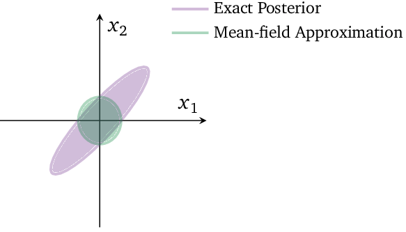
Figure 1: Taken from Blei et al.3
Since the MF models independent variables, the optimal MF variational approximation to this posterior is a product of two Gaussian distributions. The approximation has the same mean as the original density, but the covariance structure is decoupled. The KL divergence penalizes more when a distribution has more mass where does not then when has more mass than . Classical MF had its importance at the beginning, but it has multiple limitations in terms of modern and scalable applications8, which were first tackled by a combination of VI stochastic optimization and distributed computing called Stochastic Variational Inference (SVI), which I will be discussing in the next post of this series.
Appendix A
The content of this Appendix was taken from Bishop4. Standard calculus is concerned with finding derivatives of functions. We can think of a function as a mapping that takes the value of a variable as input and returns the value of the function as the output. The derivative of the function then describes how the output value varies as we make infinitesimal changes to the input value. Similarly, we can define a functional as a mapping that takes a function as the input and that returns the value of the functional as the output. We can introduce the concept of a functional derivative, which expresses how the value of the functional changes in response to infinitesimal changes to the input function. Many problems can be expressed in terms of an optimization problem in which the quantity being optimized is a functional.
The solution is obtained by exploring all possible input functions to find the one that maximizes, or minimizes, the functional. Variational methods lend themselves to finding approximate solutions by restricting the range of functions over which the optimization is performed. In the context of VI, we need to find a functional that maximizes the ELBO, thus variational inference. You can read more about variational calculus on this great Brian Keng’s blog post.
References
-
Kingma, Diederik P. Variational inference & deep learning: A new synthesis. (2017). ↩
-
Doersch, Carl. Tutorial on variational autoencoders. arXiv preprint arXiv:1606.05908 (2016). ↩
-
Blei, David M., Alp Kucukelbir, and Jon D. McAuliffe. Variational inference: A review for statisticians. Journal of the American Statistical Association 112.518 (2017): 859-877. ↩ ↩2 ↩3
-
Bishop, Christopher M. Pattern recognition and machine learning. Springer, 2006. ↩ ↩2 ↩3 ↩4
-
Murphy, Kevin P. Machine learning: a probabilistic perspective. MIT press, 2012. ↩ ↩2 ↩3
-
Bengio, Yoshua, Ian Goodfellow, and Aaron Courville. Deep learning. Vol. 1. MIT press, 2017. ↩
-
Bounded Rationality, Variational Bayes and The Mean-Field Approximation. ↩
-
Zhang, C., Butepage, J., Kjellstrom, H., & Mandt, S. Advances in variational inference. IEEE transactions on pattern analysis and machine intelligence (2018). ↩